Cox proportional hazards with correlated variables
survival-analysis
R
Published
January 22, 2024
Image by Andreas (Pixabay)
1 Introduction
Cox proportional hazards (CoxPH) model is a common approach to study the occurrence of an event as a factor of time. In medical studies, CoxPH is used to model patient survival based on disease type, gene expression, or treatment with a new drug. But CoxPH can be also used to analyze real-world business data. CoxPH analysis enables you to answer questions like:
Scientific questions:
Do female patients live longer than males?
Does drug A increase the overall patient survival time?
Does the high levels of Gene A significantly correlate with the survival outcome?
Business questions:
Do women customers spend more time in my store than men?
Which of my employees retain clients for the longest time?
Does the age of my clients correlate with their long term brand loyalty?
What is the risk of failure in the production line with the new machine compared to the old one?
One of the most powerful features of CoxPH analysis is that it allows including multiple predictors in the model, and these predictors (variables) can have different types. For instance, you can analyze continuous variables (age, gene expression, etc) along with categorical variables (male-vs-female, drug-vs-control, etc). You can also model interactions between two predictors to study complex relationships between predictors (this could be useful if you are trying to understand whether or not a drug can work function synergistically in males, for instance).
I’m in the middle of analyzing a skin cancer data set right now, and I’m trying to understand which genes correlate with the survival outcome. There are several other variables that correlate with my genes of interest (also known as problem of co-linearity), and these tend to have a bias for long-vs-short term survival. Let’s simulate a situation like this to understand how to interpret CoxPH results when there is co-linear variables.
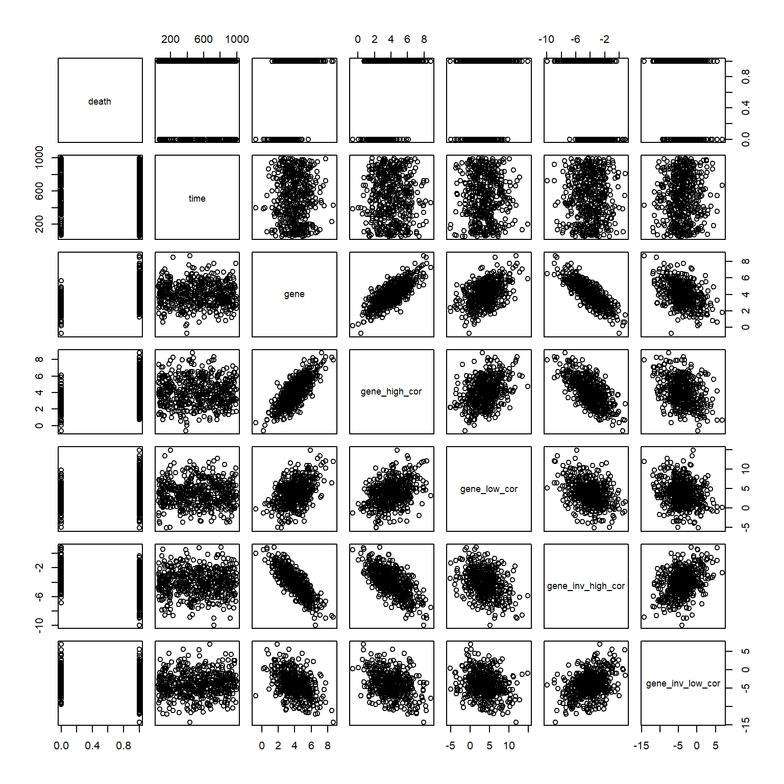
2 Simulate data
We will create a dataset with 500 observations which have survival times (time variable) between 50 and 1000 days. The death variable indicates whether or not the patient is dead at the time of measurement. 1 indicates the patient has passed, and the 0 indicates patient is still alive at that time point, but we don’t have any further information. This is called censoring, and it can happen if the patient visited the hospital at some point (ie. alive) but didn’t came back, for instance.
gene variable in the data frame shows the expression levels of an imaginary gene that is associated with increased death.
Code
# Set seed for reproducibilityset.seed(123)# Number of observationsn <-500# Max time for survival measurementmaxtime <-1000# Simulate data frame. # Sort the death and gene variables to create easy correlation# ie higher gene expressors are dying more df <-data.frame(death =sort(rbinom(n, 1, 0.75)), # 0(25%)-1(75%) distributiontime =runif(n=n, min =50, max=maxtime),gene =sort(rnorm(n, mean=4, sd=1))+rnorm(n, mean=0, sd=1))
Let’s add some positively and negatively correlated genes now. I will do that by adding some noise to the original gene variable. I created 4 different correlated variables:
gene_high_cor: High positive correlation
gene_low_cor: Low positive correlation
gene_inv_high_cor: High negative (inverse) correlation
Next step is using CoxPH. Details about the fit is given under specific columns:
coef: Regression coefficients in the log odds scale. Positive values indicate increased risk of death.
exp(coef): Hazard ratio (HR) which is equal to the exponentiated coefficient (\(e^{coef}\)). Above 1 indicates increased risk (HR=1.2 means 20% higher risk; whereas HR=0.8 means 20% reduced risk).
se(coef): Standard error of the coefficient estimate
z: Wald-statistic which is equal to coef/se(coef)
p: P-value of the estimates
Likelihood ratio test: Indicates the global p-values for rejecting the null hypothesis (ie. all of the coefficients in the model is zero) . You can see other statistics about the model by calling summary() function on the CoxPH results.
Code
library(survival)coxph(Surv(time,death) ~ gene, data = df)
Call:
coxph(formula = Surv(time, death) ~ gene, data = df)

        coef exp(coef) se(coef)     z        p
gene 0.21486   1.23969  0.03554 6.045 1.49e-09

Likelihood ratio test=35.84  on 1 df, p=2.138e-09
n= 500, number of events= 381
Code
coxph(Surv(time,death) ~ gene_high_cor, data = df)
Call:
coxph(formula = Surv(time, death) ~ gene_high_cor, data = df)

                 coef exp(coef) se(coef)     z        p
gene_high_cor 0.15365   1.16609  0.03209 4.788 1.68e-06

Likelihood ratio test=22.76  on 1 df, p=1.839e-06
n= 500, number of events= 381
Code
coxph(Surv(time,death) ~ gene_low_cor, data = df)
Call:
coxph(formula = Surv(time, death) ~ gene_low_cor, data = df)

                coef exp(coef) se(coef)     z        p
gene_low_cor 0.05600   1.05760  0.01629 3.437 0.000589

Likelihood ratio test=11.72  on 1 df, p=0.0006199
n= 500, number of events= 381
Code
coxph(Surv(time,death) ~ gene_inv_high_cor, data = df)
Call:
coxph(formula = Surv(time, death) ~ gene_inv_high_cor, data = df)

                      coef exp(coef) se(coef)      z       p
gene_inv_high_cor -0.12229   0.88489  0.02815 -4.344 1.4e-05

Likelihood ratio test=18.66  on 1 df, p=1.56e-05
n= 500, number of events= 381
Code
coxph(Surv(time,death) ~ gene_inv_low_cor, data = df)
Call:
coxph(formula = Surv(time, death) ~ gene_inv_low_cor, data = df)

                     coef exp(coef) se(coef)      z        p
gene_inv_low_cor -0.06808   0.93418  0.01635 -4.165 3.12e-05

Likelihood ratio test=17.45  on 1 df, p=2.946e-05
n= 500, number of events= 381
4 Multivariable CoxPH analysis
After seeing how the result looks like above, next I’d like to try survival modeling using other correlated predictors alone or in combination with each other.
4.1 gene + gene_high_cor
Code
# covariable in combocoxph(Surv(time,death) ~ gene + gene_high_cor, data = df)
Call:
coxph(formula = Surv(time, death) ~ gene + gene_high_cor, data = df)

                 coef exp(coef) se(coef)     z       p
gene          0.20482   1.22731  0.05652 3.624 0.00029
gene_high_cor 0.01150   1.01157  0.05038 0.228 0.81939

Likelihood ratio test=35.9  on 2 df, p=1.604e-08
n= 500, number of events= 381
4.2 gene + gene_low_cor
Code
# covariable in combocoxph(Surv(time,death) ~ gene + gene_low_cor, data = df)
Call:
coxph(formula = Surv(time, death) ~ gene + gene_low_cor, data = df)

                coef exp(coef) se(coef)     z        p
gene         0.20134   1.22304  0.04078 4.938 7.91e-07
gene_low_cor 0.01230   1.01237  0.01840 0.668    0.504

Likelihood ratio test=36.29  on 2 df, p=1.317e-08
n= 500, number of events= 381
4.3 gene_high_cor + gene_low_cor
Code
# covariables in combocoxph(Surv(time,death) ~ gene_high_cor + gene_low_cor, data = df)
Call:
coxph(formula = Surv(time, death) ~ gene_high_cor + gene_low_cor,
    data = df)

                 coef exp(coef) se(coef)     z        p
gene_high_cor 0.13049   1.13939  0.03431 3.803 0.000143
gene_low_cor  0.03223   1.03276  0.01738 1.855 0.063579

Likelihood ratio test=26.19  on 2 df, p=2.056e-06
n= 500, number of events= 381
4.4 gene + gene_inv_high_cor
Code
# covariable in combocoxph(Surv(time,death) ~ gene + gene_inv_high_cor, data = df)
Call:
coxph(formula = Surv(time, death) ~ gene + gene_inv_high_cor,
    data = df)

                     coef exp(coef) se(coef)     z        p
gene              0.27951   1.32248  0.06439 4.341 1.42e-05
gene_inv_high_cor 0.06172   1.06366  0.05146 1.199     0.23

Likelihood ratio test=37.29  on 2 df, p=7.998e-09
n= 500, number of events= 381
4.5 gene + gene_inv_low_cor
Code
# covariable in combocoxph(Surv(time,death) ~ gene + gene_inv_low_cor, data = df)
Call:
coxph(formula = Surv(time, death) ~ gene + gene_inv_low_cor,
    data = df)

                     coef exp(coef) se(coef)      z        p
gene              0.18481   1.20299  0.04044  4.570 4.88e-06
gene_inv_low_cor -0.02845   0.97195  0.01842 -1.544    0.123

Likelihood ratio test=38.23  on 2 df, p=4.983e-09
n= 500, number of events= 381
4.6 gene_inv_high_cor + gene_inv_low_cor
Code
# covariables in combocoxph(Surv(time,death) ~ gene_inv_high_cor + gene_inv_low_cor, data = df)
Call:
coxph(formula = Surv(time, death) ~ gene_inv_high_cor + gene_inv_low_cor,
    data = df)

                      coef exp(coef) se(coef)      z       p
gene_inv_high_cor -0.09271   0.91146  0.03033 -3.057 0.00224
gene_inv_low_cor  -0.04936   0.95184  0.01745 -2.829 0.00467

Likelihood ratio test=26.68  on 2 df, p=1.606e-06
n= 500, number of events= 381
4.7 gene_high_cor + gene_inv_high_cor
Code
# covariables in combocoxph(Surv(time,death) ~ gene_high_cor + gene_inv_high_cor, data = df)
Call:
coxph(formula = Surv(time, death) ~ gene_high_cor + gene_inv_high_cor,
    data = df)

                      coef exp(coef) se(coef)      z      p
gene_high_cor      0.10934   1.11554  0.04239  2.579 0.0099
gene_inv_high_cor -0.05931   0.94241  0.03714 -1.597 0.1103

Likelihood ratio test=25.31  on 2 df, p=3.194e-06
n= 500, number of events= 381
4.8 All covariables together
Code
formula_pred <-formula(paste("Surv(time,death) ~",paste(grep("gene", colnames(df), value =T),collapse =" + ") ) )# covariables in combocoxph(formula_pred, data = df)
Call:
coxph(formula = formula_pred, data = df)

                       coef exp(coef)  se(coef)      z      p
gene               0.217201  1.242594  0.085836  2.530 0.0114
gene_high_cor      0.015962  1.016091  0.050472  0.316 0.7518
gene_low_cor       0.009508  1.009553  0.018484  0.514 0.6070
gene_inv_high_cor  0.053296  1.054742  0.052402  1.017 0.3091
gene_inv_low_cor  -0.027322  0.973048  0.018442 -1.481 0.1385

Likelihood ratio test=39.8  on 5 df, p=1.635e-07
n= 500, number of events= 381
4.9 All covariables made random and modelled together
Note
You will see why I’m doing this in the next section.
Code
# make all covariables randomdf[, 4:ncol(df)] <-rnorm(n*(ncol(df)-3), mean =20, sd =10)# covariables in combocoxph(formula_pred, data = df)
Call:
coxph(formula = formula_pred, data = df)

                        coef  exp(coef)   se(coef)      z        p
gene               2.172e-01  1.243e+00  3.580e-02  6.069 1.29e-09
gene_high_cor     -5.234e-03  9.948e-01  5.211e-03 -1.004    0.315
gene_low_cor      -9.997e-05  9.999e-01  5.430e-03 -0.018    0.985
gene_inv_high_cor -6.686e-03  9.933e-01  4.841e-03 -1.381    0.167
gene_inv_low_cor   3.418e-03  1.003e+00  5.076e-03  0.673    0.501

Likelihood ratio test=39.02  on 5 df, p=2.35e-07
n= 500, number of events= 381
5 Take home point
Not unexpectedly, when there are correlated variables in the survival model, the coefficients of individual predictors can change depending on what enters the model. Let’s try to digest this a bit. In our simulated example, variable gene is closely associated with the survival outcome (ie. patients with high gene are dying more ). The other covariables are generated so that they are correlated with the variable gene, but there is no mathematical relationship between these covariables and the survival outcome. In other words, higher levels of gene go in parallel with higher chances for observing death = 1. After capturing this relationship, the addition of random noise to gene to obtain gene_high_cor (and other covariables) does not explain the changes vital status any further. You might have two correlated variables gene and gene_high_cor for example, but only one of them may be associated with the survival outcome whereas the other one is just a derivative of the first one.
This is why you see a “significant” HR value of 1.16609 in the univariable model involving gene_high_cor in Section 3 (keep in mind that this covariable is positively correlated with the variable of interest, gene); but this significance goes away when you model gene_high_cor together with gene in Section 4.1. The same can be said for multivariable analyses involving other covariables.
Finally, when you model all predictors together in Section 4.8, you see that the HR values of all the covariables converge to 1 (ie. no effect on survival) whereas HR value of gene is 1.242594. However, when you look at the p-value, albeit it is still significant (as defined by < 0.05), you’ll see that it is higher now compared to univariable analysis. This may be happening because our covariables could still explain vital status changes at least somewhat. To support this notion, when we made all covariables random and performed survival modeling in Section 4.9, the coefficient and the p-value of gene looked quite similar to the univariable model in Section 3. I hope this post helped you wraped your mind around how CoxPH works when there are correlated variables involved.