Many statistical analysis packages in R utilize design matrices for setting up comparisons between data subsets. The two Bioconductor packages most commonly used for transcriptomics data analysis, DESeq2 and limma, are no exception. Although the design matrices and contrasts are intuitive to understand for simple cases, things can get confusing when more complex multi-factorial studies are involved. You can find dozens of questions asked on Biostars and Bioconductor forums seeking for help in this matter.
To be fair, the DESeq2 and limma vignettes have dedicated sections explaining designs and contrasts, but I found these not very easy to follow the first time I saw them. In this note-to-self (and to-my-students) post, I intend to explain how to construct designs in various study contexts and access specific comparisons of interest using DESeq2. I benefited greatly from the DESeq2 vignette itself and the tutorial writted by Hugo Tavares. The visuals embedded in this post are adapted from the accompanying slide show to Hugo Tavares’ tutorial.
I will start with the simplest case where there are only two groups to be compared (i.e. one factor, two levels). Here, I will discuss different ways of constructing the design matrix and accessing the results. Then, I will exemplify a scenario with three groups (i.e. one factor, three levels) apply the approaches we discussed in the first case. Lastly, we will see an example involving 4 groups (i.e. two factors, two levels each) and something more complicated although conceptually it will be very similar. So, here goes nothin’…
1 One experimental condition, two groups
This is a classic case where you might have a treatment group and a control group, and you are interested in figuring out how the treatment affects the gene expression. This type of data is referred to in vignettes as “one factor two levels”.
1.1 Simulate data
Code
# for reproducibilityset.seed(1)suppressPackageStartupMessages(library(DESeq2))# simulate datadds1 <-makeExampleDESeqDataSet(n =1000, m =6, betaSD =2)dds1$condition <-factor(rep(c("treatment", "control"), each =3))# observe the samples and groupscolData(dds1)
DataFrame with 6 rows and 1 column
        condition
         <factor>
sample1 treatment
sample2 treatment
sample3 treatment
sample4 control
sample5 control
sample6 control
1.2 Contrasts from design with intercept
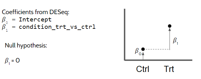
When we use the formula ~ condition the model matrix is set up with an intercept, that is, the first level of the condition is considered as the reference group. Since R orders factor levels based on the alphabetical order, in our case, control will be the reference. The order can be explicitly changed using relevel() or factor(..., levels=c(...)), if needed.
Here, the gene expression is modeled as seen below where \(\beta_0\) is the intercept and \(\beta_1\) is the coefficient for the treatment’s effect:
\[
Expression = \beta_0 + \beta_1CondTreatment
\]
We can directly get the results we are interested in using the contrasts argument as seen below. contrasts argument can accept a number of inputs:
A character vector with exactly three elements: the name of a factor in design formula (eg. “condition” in our case), the name of the numerator (ie. group of interest, “treatment” in our case), and the name of the denominator (ie. reference group, “control” in our case). This would look like this for our example: c("condition", "treatment", "control"))
A list of two character vectors: the names of the fold changes for the numerator, and the names of fold changes for the denominator. This approach allows you to group comparisons together in the numerator and denominator for extracting specific comparisons (more below). In our case we only have one comparison, which is condition_treatment_vs_control, so we will provide it alone as list(condition_treatment_vs_control). Note that these names came from the colData in dds object automatically.
Code
# design with intercept (control group is the intercept, or the reference)design(dds1) <-~ condition# note the zeros for under treatment for samples 4-6model.matrix(~condition, colData(dds1))
# differential expression analysisdds1 <-DESeq(dds1)# see the comparisonsresultsNames(dds1)
[1] "Intercept" "condition_treatment_vs_control"
Code
res <-results(dds1, contrast =list("condition_treatment_vs_control"))# res <- results(dds1, contrast = c("condition", "treatment", "control")) # alternatively# res
1.3 Contrasts from design without intercept
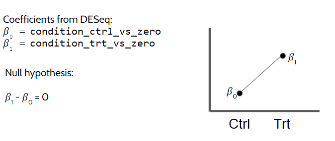
Sometimes it is easier to work with no-reference designs. You can tell the algorithm not to have an intercept (ie. control group) by using ~ 0 + condition formula. The way you specify the contrast argument will change, but the results will be identical with the first case. You may not see the benefit of using this approach in this simple example, but when multiple factors and factor levels are involved, it may be easier to construct no-intercept designs.
This is how a zero-intercept model looks like:
\[
Expression = \beta_0 Control + \beta_1 Treatment
\]
NOTE: When you have two factors in your data and use no-intercept design, you will have no reference group for the first factor (as seen here), but for the second factor a reference group is still defined. Although this is sensible, I find it somewhat confusing when it comes to specifying contrasts for specific pairwise comparisons. But the next section will help out with this.
Code
dds2 <- dds1# design without intercept (no reference)design(dds2) <-~0+ condition# note the zeros for under treatment for samples 4-6model.matrix(~0+condition, colData(dds2))
# differential expression analysisdds2 <-DESeq(dds2)# see the comparisonsresultsNames(dds2)
[1] "conditioncontrol" "conditiontreatment"
Code
res <-results(dds2, contrast =list("conditiontreatment", "conditioncontrol"))# res
Above you see that we are providing list("conditiontreatment", "conditioncontrol") to contrasts argument. This way, we are telling the algorithm to take fold changes of differentially expressed genes in the conditiontreatment (differential expression is measured against the hypothetical zero) and divide that by the log fold changes of conditioncontrol. Thus you get the treatment vs control:
The results should be equivalent between the first the second design. Conceptually, the zero intercept model in DESeq2 does not compare conditions against each other, instead, each condition’s coefficient represents its own log2-fold expression estimate relative to zero.
1.4 A new approach for defining contrasts
It was easy to specify the contrasts in the examples above, but Mike Love and Hugo Tavares shares an interesting way of generalizing this concept, which is especially useful for more complex designs. This approach works for designs with or without an intercept. This approach involves three steps:
Getting the model matrix
Subsetting the matrix for each group of interest and calculate its column means - this results in a vector of coefficients for each group
Subtracting the group vectors from each other according to the comparison we’re interested in
The resulting object is a numeric vector specifying the groups in comparison.
Code
# get the model matrixmod_mat <-model.matrix(design(dds1), colData(dds1))mod_mat
res <-results(dds1, contrast = treatment - control)
The code may look overly complex to get a simple numeric vector to specify groups to compare. In this example, it is maybe so. But when there is a more complex experimental setup and you are comparing various subgroups, this can be helpful. Hugo Tavares created a function in a GitHub Gist to facilitate contrasts. But here I wanted to improve on that to avoid creation of unneccessary objects in the global environment and allow more complex contrasts.
The contraster() function below allows the user to extract contrasts from the DESeq object after specifying custom groups. group1 and group2 arguments can take lists of character vectors each having 2 or more items. The first item of the character vector should point to one of the columns in the colData(dds), that is the grouping variable. The second item of the character vector (and onwards) should be the sample subgroups to be included in the analysis. The differences are calculating subtracting group2 from group1. Read on for a discussion on the weighted argument.
Code
contraster <-function(dds, # should contain colData and design group1, # list of character vectors each with 2 or more items group2, # list of character vectors each with 2 or more itemsweighted = F){ mod_mat <-model.matrix(design(dds), colData(dds)) grp1_rows <-list() grp2_rows <-list()for(i in1:length(group1)){ grp1_rows[[i]] <-colData(dds)[[group1[[i]][1]]] %in% group1[[i]][2:length(group1[[i]])] }for(i in1:length(group2)){ grp2_rows[[i]] <-colData(dds)[[group2[[i]][1]]] %in% group2[[i]][2:length(group2[[i]])] } grp1_rows <-Reduce(function(x, y) x & y, grp1_rows) grp2_rows <-Reduce(function(x, y) x & y, grp2_rows) mod_mat1 <- mod_mat[grp1_rows, ,drop=F] mod_mat2 <- mod_mat[grp2_rows, ,drop=F]if(!weighted){ mod_mat1 <- mod_mat1[!duplicated(mod_mat1),,drop=F] mod_mat2 <- mod_mat2[!duplicated(mod_mat2),,drop=F] }return(colMeans(mod_mat1)-colMeans(mod_mat2))}
We can use this new function to get the exact results from before:
Code
res <-results(dds1, contrast =contraster(dds1, group1 =list(c("condition", "treatment")), group2 =list(c("condition", "control"))))
So far we have learned a simple two-group analysis. We will next use these in more complex experimental contexts.
2 One experimental condition, three levels
This is a classic case when you have a control group and two treatment groups (e.g. treatmentA and treatmentB). From now on, I will be using designs with intercepts. Let’s see how things work.
2.1 Simulate data
In this design the gene expression is modeled as follows where \(\beta_0\) is the intercept, \(\beta_1\) is the coefficient (effect) of treatmentA, and the \(\beta_2\) is the coefficient of treatmentB:
Now we have three coefficients: 1) control group as intercept, 2) TreatmentA vs control, 3) TreatmentB vs control. We can get different results as follows:
Code
# treatmentA vs controlres1 <-results(dds3, contrast =list("condition_treatmentA_vs_control"))# treatmentB vs controlres2 <-results(dds3, contrast =list("condition_treatmentB_vs_control"))# treatmentA vs treatmentBres3 <-results(dds3, contrast=list("condition_treatmentA_vs_control","condition_treatmentB_vs_control"))
Or we can alternatively use our new function as well:
Code
# Alternatively we can use our new functionres1 <-results(dds3,contrast =contraster(dds3,group1 =list(c("condition","treatmentA")),group2 =list(c("condition", "control"))))res2 <-results(dds3,contrast =contraster(dds3,group1 =list(c("condition","treatmentB")),group2 =list(c("condition", "control"))))res3 <-results(dds3,contrast =contraster(dds3,group1 =list(c("condition","treatmentA")),group2 =list(c("condition", "treatmentB"))))
This function also allows us to perform more customized analyses. For instance, if you are trying to compare treatment groups as a whole (treatmentA and treatmentB combined) against reference, you would need to write group1 = list(c("condition", "treatmentA", "treatmentB")) and group2 = list(c("condition", "control"). The analysis will be performed by subtracting group2 from group1, that is you are comparing the average of the treatment groups to the control.
Let’s see how the contrast is set up in this approach. As you can see below, each treatment group has a weight of 0.5, that is, their average is being compared against the control group.
If the groups were unbalanced, by setting weighted = TRUE, you can assign weights according to group sizes. However, there are GitHub issues on the matter (1, 2, 3) pointing out that this approach may be flawed where replicates don’t occur in all subgroups and numbers of replicates are different. You can see the behavior of contraster function by creating an unbalanced data set:
Code
# Convert the last control to treatmentAdds3$condition[3] <-"treatmentA"contraster(dds3, group1 =list(c("condition", "treatmentA", "treatmentB")),group2 =list(c("condition", "control")),weighted =TRUE)
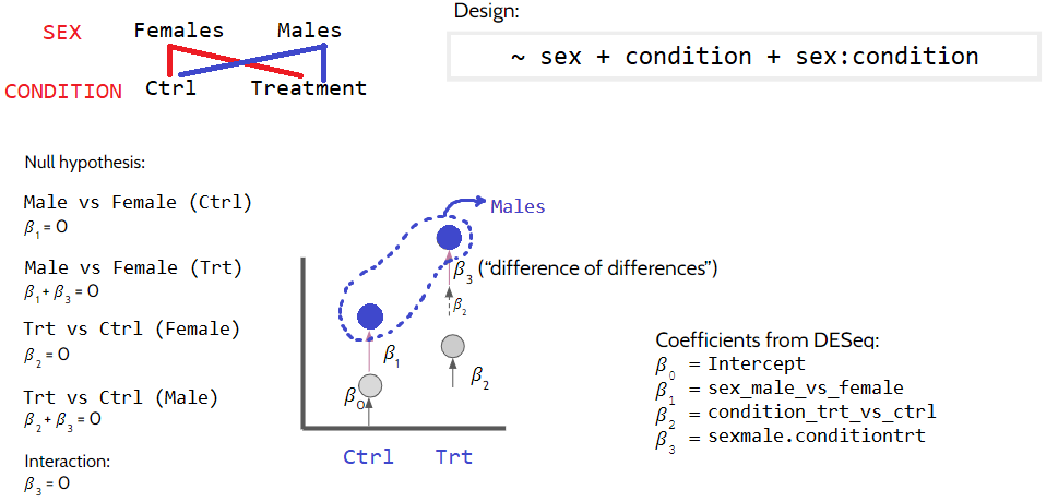
In some experiments grouping variables may interact with one another. An example for this can be that a treatment affects males and females differently. In this case we are looking at something like this:
3.1 Simulate data
Code
dds4 <-makeExampleDESeqDataSet(n =1000, m =12, betaSD =2)dds4$sex <-factor(rep(c("female", "male"), each =6))dds4$condition <-factor(rep(c("treatment", "control"), 6))dds4 <- dds4[, order(dds4$sex, dds4$condition)]colnames(dds4) <-paste0("sample", 1:ncol(dds4))design(dds4) <-~ sex + condition + sex:conditiondds4 <-DESeq(dds4)resultsNames(dds4)
3.2.5 Interaction between sex and condition (i.e. do males and females respond differently to the treatment?)
This will be a little more wordy, because we are trying to get the “difference of the differences”. For this analysis, we are interested in genes that are differentially expressed in males in treatment condition, but not in the control condition (ie. genes uniquely changing in males due to treatment). In other words, we are isolating \(\beta_3\) by doing the following:
# I am not sure why one would like to weight contrasts in this example# See the issues #7 and #11 in the Hugo Tavares GitHub repocontraster(dds,group1=list(c("batch", 1), c("sex", "male"), c("condition", "treatmentB", "treatmentA")),group2=list(c("batch", 1), c("sex", "male"), c("condition", "control")), weighted = T)